How to generate a utility report?#
Check that the synthetic data preserve the information of the real data#
Assume that the synthetic data is already generated
Based on the Wisconsin Breast Cancer Dataset
[1]:
# Standard library
import sys
import tempfile
from pathlib import Path

sys.path.append("..")

# 3rd party packages
import pandas as pd

# Local packages
import config
import utils.draw
from metrics.utility.report import UtilityReport
Load the real and synthetic WBCD datasets#
[2]:
df_real = {}
df_real["train"] = pd.read_csv(
    "../data/" + config.WBCD_DATASET_TRAIN_FILEPATH.stem + ".csv"
)
df_real["test"] = pd.read_csv(
    "../data/" + config.WBCD_DATASET_TEST_FILEPATH.stem + ".csv"
)
df_real["train"].shape
[2]:
(359, 10)
Choose the synthetic dataset#
[3]:
df_synth = {}  # generated by Synthpop ordered here
df_synth["train"] = pd.read_csv("../results/data/2023-07-31_Synthpop_359samples.csv")
df_synth["test"] = pd.read_csv("../results/data/2023-07-31_Synthpop_90samples.csv")
df_synth["test"].shape
[3]:
(90, 10)
Configure the metadata dictionary#
The continuous and categorical variables need to be specified, as well as the variable to predict for the future learning task#
[4]:
metadata = {
    "continuous": [
        "Clump_Thickness",
        "Uniformity_of_Cell_Size",
        "Uniformity_of_Cell_Shape",
        "Marginal_Adhesion",
        "Single_Epithelial_Cell_Size",
        "Bland_Chromatin",
        "Normal_Nucleoli",
        "Mitoses",
        "Bare_Nuclei",
    ],
    "categorical": ["Class"],
    "variable_to_predict": "Class",
}
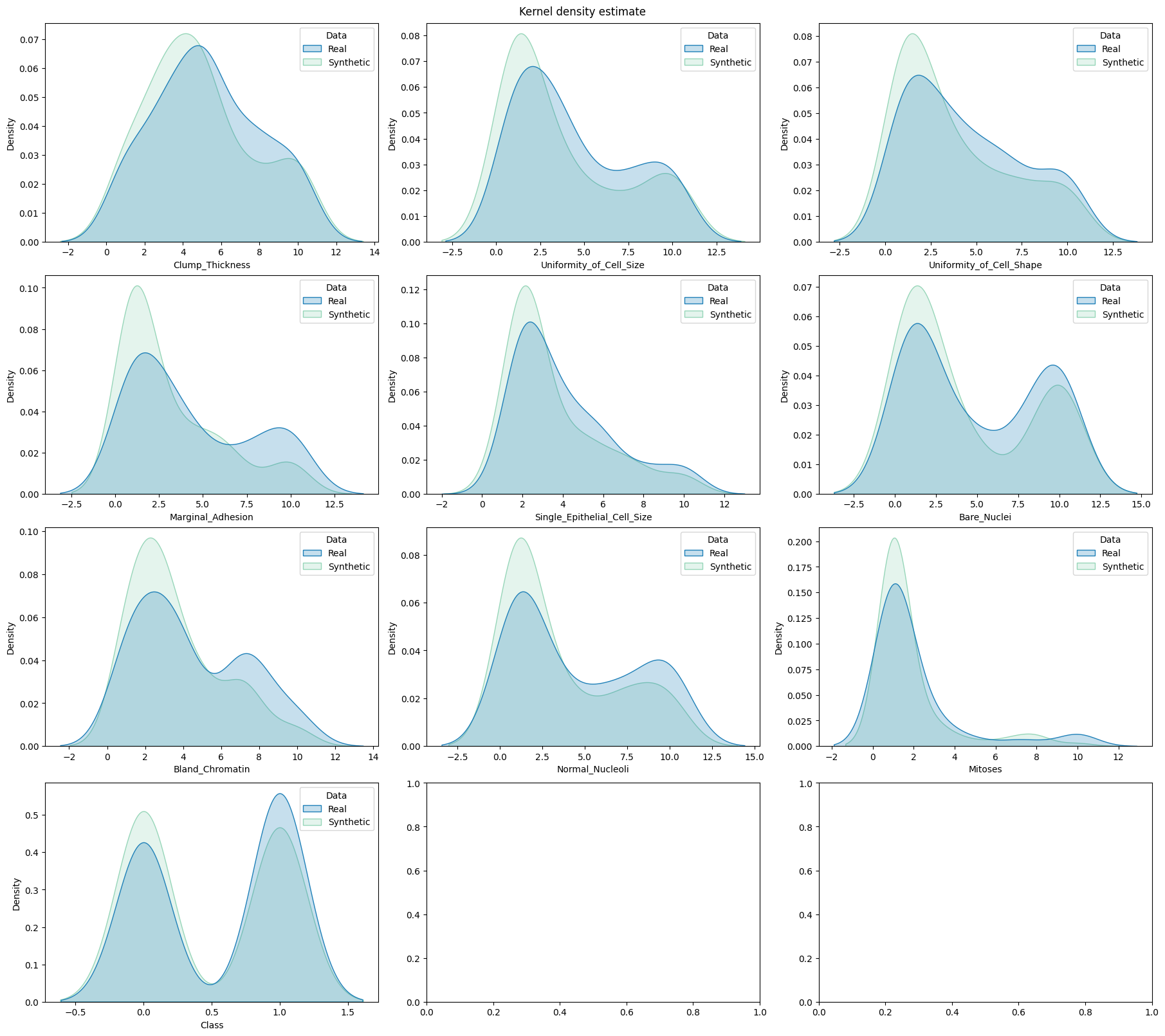
Compare the distributions#
[5]:
import matplotlib.pyplot as plt

fig, axes = plt.subplots(  # manually set number of cols/rows
    nrows=4, ncols=3, squeeze=0, figsize=(18, 16), layout="constrained"
)
axes = axes.reshape(-1)
utils.draw.kde_plot_hue_plot_per_col(
    df=df_real["test"],
    df_nested=df_synth["test"],
    original_name="Real",
    nested_name="Synthetic",
    hue_name="Data",
    title="Kernel density estimate",
    axes=axes,
)
Generate the utility report#
Some metrics will not be computed since the only categorical variable is the variable to predict
1. First option: Create and compute the full utility report - it takes some time#
[6]:
report = UtilityReport(
    dataset_name="Wisconsin Breast Cancer Dataset",
    df_real=df_real,
    df_synthetic=df_synth,
    metadata=metadata,
    figsize=(8, 6),  # will be automatically adjusted for larger or longer figures
    random_state=0,  # for reproducibility purposes
    report_filepath=None,  # load a computed report if available
    metrics=None,  # list of the metrics to compute. If not specified, all the metrics are computed.
    cross_learning=True,  # not parallelized yet, can be set to False if the computation is too slow. See the use_gpu flag to accelerate the computation
    num_repeat=1,  # for the metrics relying on predictions to account for randomness
    num_kfolds=3,  # the number of folds to tune the hyperparameters for the metrics relying on predictors
    num_optuna_trials=20,  # the number of trials of the optimization process for tuning hyperparameters for the metrics relying on predictors
    use_gpu=True,  # run the learning tasks on the GPU
    alpha=0.05,  # for the pairwise chi-square metric
)
[7]:
report.compute()
Get the summary report as a pandas dataframe#
[8]:
report.specification()
----- Wisconsin Breast Cancer Dataset -----
Contains:
    - 359 instances in the train set,
    - 90 instances in the test set,
    - 10 variables, 9 continuous and 1 categorical.
[9]:
df_summary = report.summary()
[10]:
by = ["name", "objective", "min", "max"]
df_summary.groupby(by).apply(lambda x: x.drop(by, axis=1).reset_index(drop=True))
[10]:
| alias | submetric | value | |||||
|---|---|---|---|---|---|---|---|
| name | objective | min | max | ||||
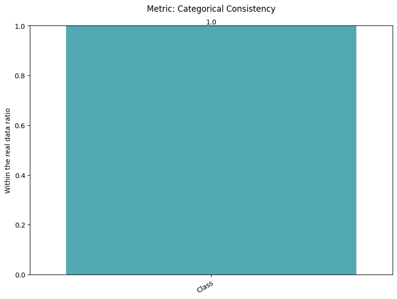
| Categorical Consistency | max | 0 | 1.0 | 0 | cat_consis | within_ratio | 1.000000 |
| Categorical Statistics | max | 0 | 1.0 | 0 | cat_stats | support_coverage | 1.000000 |
| 1 | cat_stats | frequency_coverage | 0.958217 | ||||
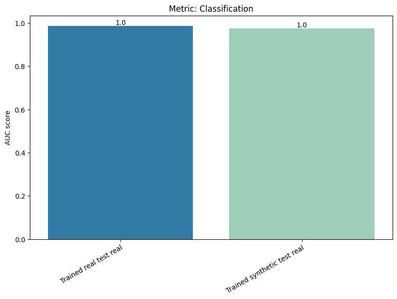
| Classification | min | 0 | 1.0 | 0 | classif | diff_real_synth | 0.011061 |
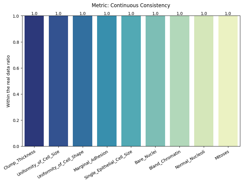
| Continuous Consistency | max | 0 | 1.0 | 0 | cont_consis | within_ratio | 1.000000 |
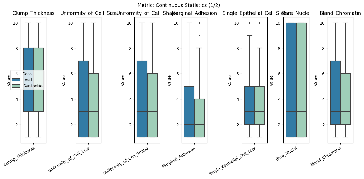
| Continuous Statistics | min | 0 | inf | 0 | cont_stats | median_l1_distance | 0.012346 |
| 1 | cont_stats | iqr_l1_distance | 0.061728 | ||||
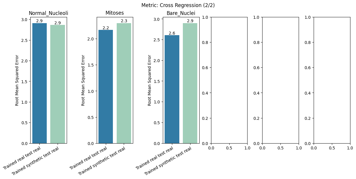
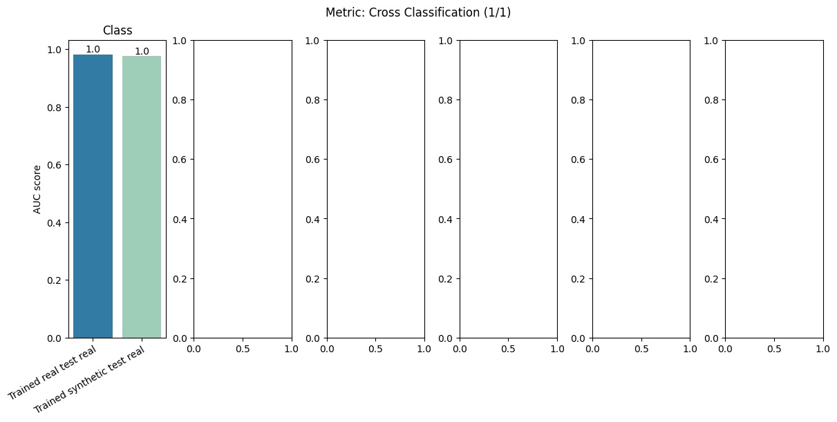
| Cross Classification | min | 0 | 1.0 | 0 | cross_classif | diff_real_synth | 0.006033 |
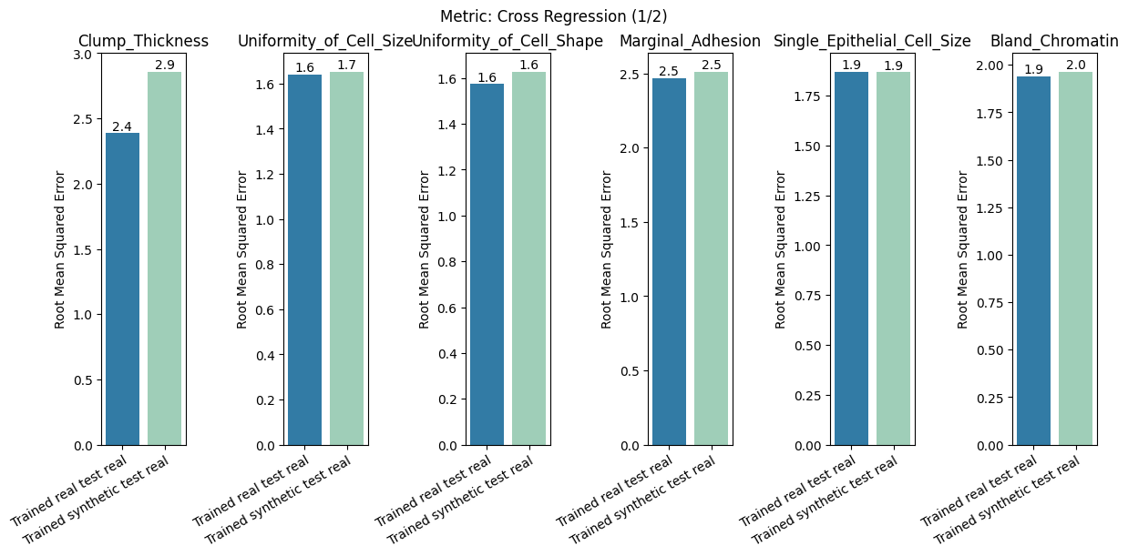
| Cross Regression | min | 0 | inf | 0 | cross_reg | diff_real_synth | 0.120401 |
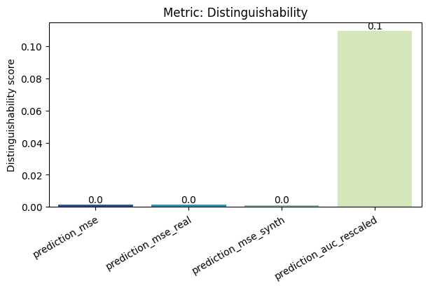
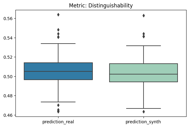
| Distinguishability | min | 0 | 1.0 | 0 | dist | prediction_mse | 0.001273 |
| 1 | dist | prediction_mse_real | 0.001356 | ||||
| 2 | dist | prediction_mse_synth | 0.001189 | ||||
| 3 | dist | prediction_auc_rescaled | 0.109506 | ||||
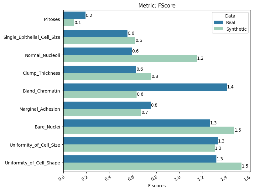
| FScore | min | 0 | inf | 0 | fscore | diff_f_score | 0.241306 |
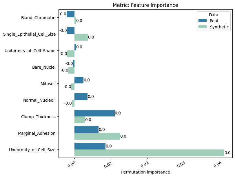
| Feature Importance | min | 0 | inf | 0 | feature_imp | diff_permutation_importance | 0.007363 |
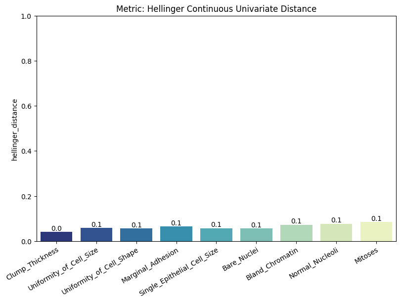
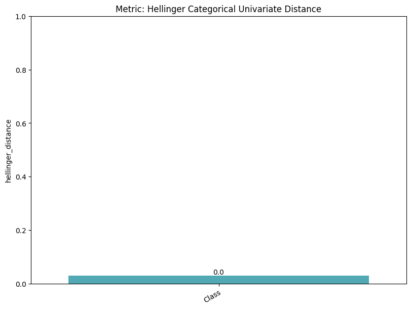
| Hellinger Categorical Univariate Distance | min | 0 | 1.0 | 0 | hell_cat_univ_dist | hellinger_distance | 0.029553 |
| Hellinger Continuous Univariate Distance | min | 0 | 1.0 | 0 | hell_cont_univ_dist | hellinger_distance | 0.062990 |
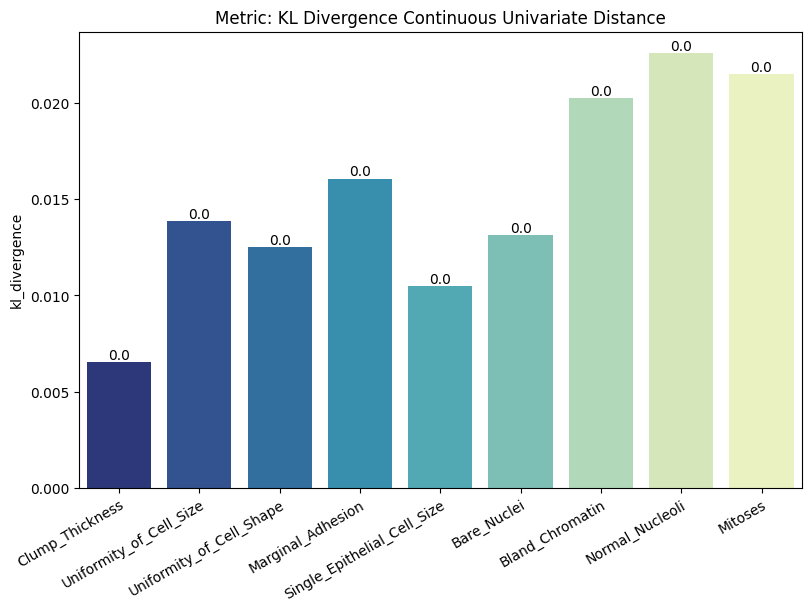
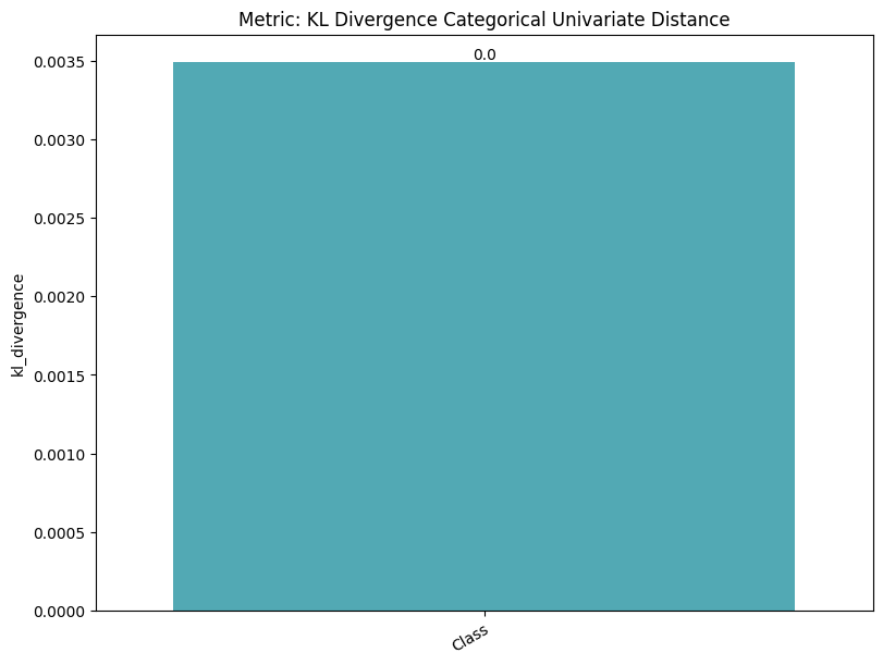
| KL Divergence Categorical Univariate Distance | min | 0 | inf | 0 | kl_div_cat_univ_dist | kl_divergence | 0.003493 |
| KL Divergence Continuous Univariate Distance | min | 0 | inf | 0 | kl_div_cont_univ_dist | kl_divergence | 0.015213 |
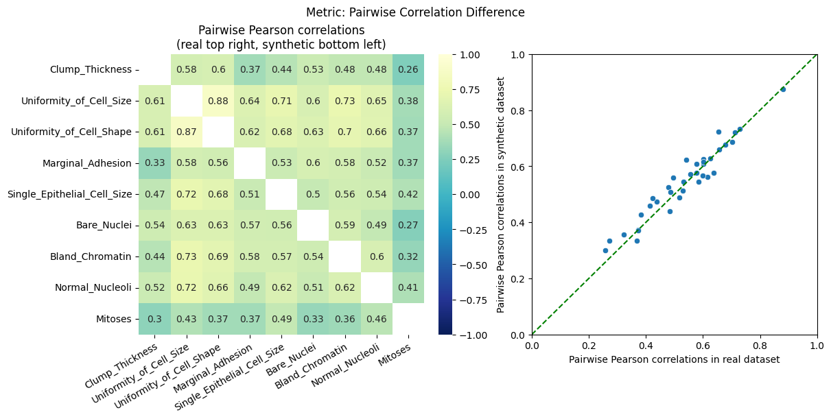
| Pairwise Correlation Difference | min | 0 | inf | 0 | pcd | norm | 0.316965 |
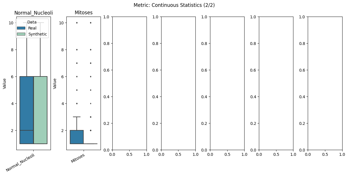
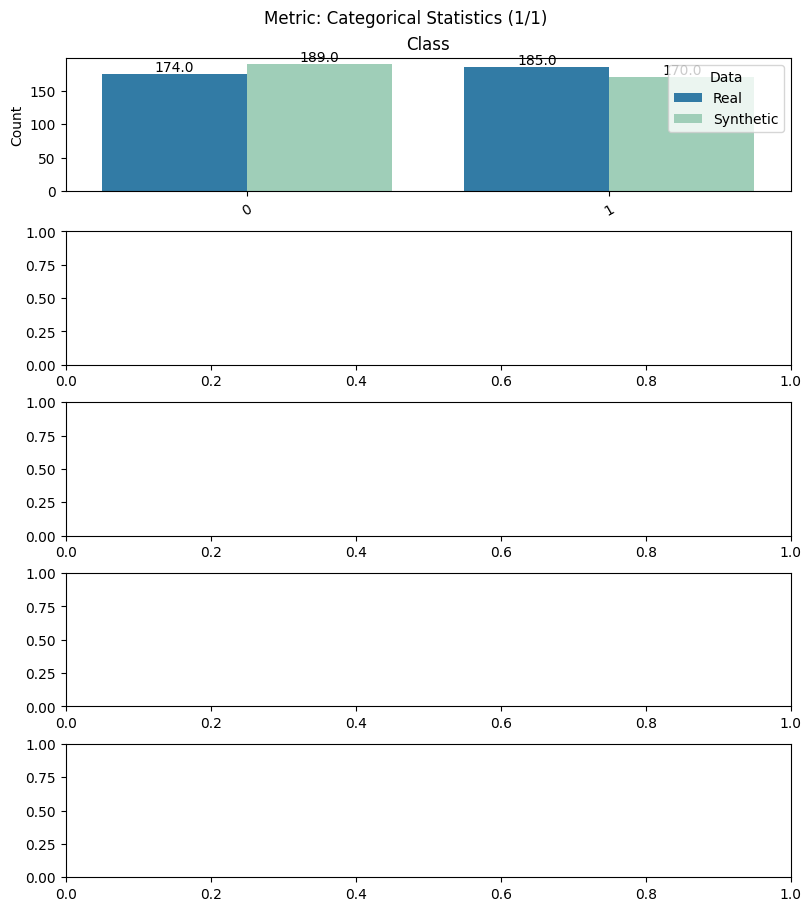
Display the detailed report#
[11]:
report.detailed(show=True, save_folder=None, figure_format="png")
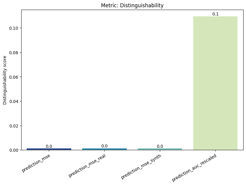

To display only one metric, the draw function can be used.#
[12]:
report.draw(
    metric_name="Distinguishability",
    figsize=(
        6,
        4,
    ),  # Reset here the size of the figure if it was too small in the report
    show=True,
    save_folder=None,
    figure_format="png",
)
Save and load the report#
[13]:
with tempfile.TemporaryDirectory() as temp_dir:
    report.save(savepath=temp_dir, filename="utility_report")  # save
    new_report = UtilityReport(
        report_filepath=Path(temp_dir) / "utility_report.pkl"
    )  # load
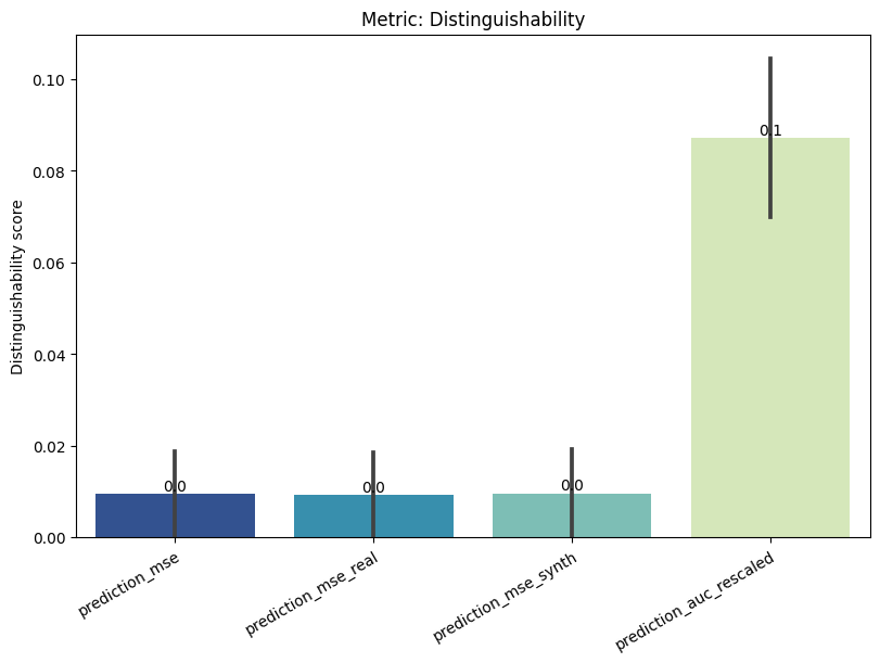
2. Second option: Create and compute the report for a subset of metrics only#
Here only compute the Distinguishability metric#
[14]:
report = UtilityReport(
    dataset_name="Wisconsin Breast Cancer Dataset",
    df_real=df_real,
    df_synthetic=df_synth,
    metadata=metadata,
    metrics=["Distinguishability"],  # the subset of metrics to compute
    num_repeat=2,
    num_kfolds=3,
    num_optuna_trials=20,
    use_gpu=False,  # if a GPU is available, it will accelerate the computation
    alpha=0.05,
)
[15]:
report.compute()
[16]:
report.summary()
[16]:
| name | alias | submetric | value | objective | min | max | |
|---|---|---|---|---|---|---|---|
| 0 | Distinguishability | dist | prediction_mse | 0.009470 | min | 0 | 1.0 |
| 1 | Distinguishability | dist | prediction_mse_real | 0.009290 | min | 0 | 1.0 |
| 2 | Distinguishability | dist | prediction_mse_synth | 0.009650 | min | 0 | 1.0 |
| 3 | Distinguishability | dist | prediction_auc_rescaled | 0.087222 | min | 0 | 1.0 |
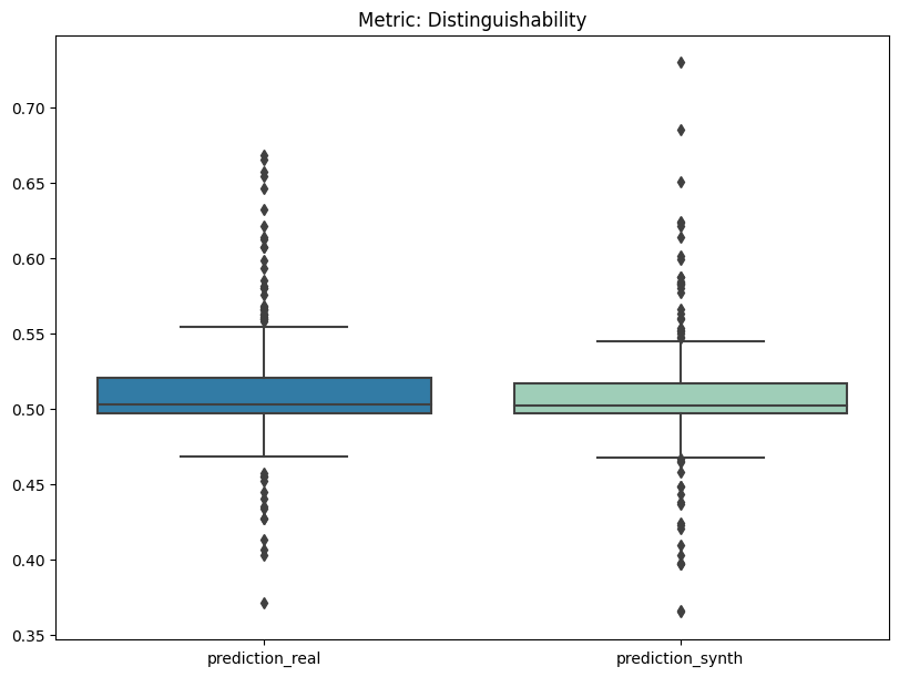
[17]:
report.detailed(show=True, save_folder=None, figure_format="png")
[ ]: